(Class 6) Part 5 contd: Data summarizing, reshaping, and wrangling with multiple tables (contd)
R Project files
In this class we will finish the part5 material from this folder link. There are a couple updates so please download part5_updated.Rmd and part5_haven.Rmd.
This year’s class video
See Slack for the zoom recording link (though zoom had some malfunction that failed to show the correct Rstudio screen, so last year’s video may be more helpful)
Last Year’s Class Video (Part 5 continued, split about the same)
View last year’s class and materials here.
Post-Class
Please fill out the following survey and we will discuss the results during the next lecture. All responses will be anonymous.
- Clearest Point: What was the most clear part of the lecture?
- Muddiest Point: What was the most unclear part of the lecture to you?
- Anything Else: Is there something you’d like me to know?
Muddiest Points
Somewhat equal numbers said that pivot/joining were clear or were muddy! I think that sounds about right, though, these concepts are tricky and will take a lot of practice. Today’s class will use these methods again and I hope that will help solidify what you’ve learned.
I really do recommend watching the short video that I recommended last class if you’re still having trouble with grasping pivoting.
Dr. Kelly Bodwin’s Reshaping Data Video
For a short version, watch the pivot_longer excerpt about “working backwards” from a plot. Then watch the pivot_wider excerpt
Also read this join cheatsheet for some good explanations/examples about which join to use when!
The rstudio cheatsheet is also good.
Definitely do the readings in the R for Data Science in the appropriate chapters as well! joining, pivoting
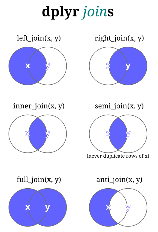
For the different join types, here are some visuals I find helpful.
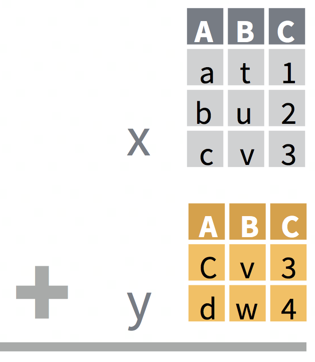
When we use bind_rows() we stack cases on top of each other like so:

For joins, we put columns next to each other based on matching keys. The “intersection” of keys is shown in these diagrams for each type of join, with the blue denoting which keys/rows we keep from which table:

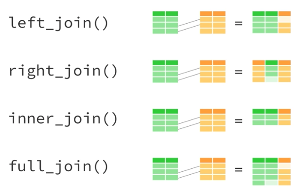
A more data oriented visual is shown below. The lines denote the keys that match:

This is from the part5 Rmd:
When do we use which join?
See this two-table verbs vignette and this cheatsheet for some extra explanations.
These joins are created to match SQL joins for databases.
inner_join= You only want data that is in both tablesleft_join= You only want data that is in one table.- Often the right table is a subset of the left table, so it’s easy to use this to keep everything in the bigger table, and join on the smaller table
- If the left table contains a cohort of interest, i.e. everyone that has been given a specific treatment, and you want to get their lab values from another table, use
left_join()to add those lab values in the cohort defined by the left table
right_join= maybe neverright_joindoes the same thing asleft_joinbut backwards, I find left join easier to think about (personal preference)
full_join= does not remove any rows, you might want to use this as your default and filter lateranti_joinandsemi_join= filtering joins, probably use rarely, use right table as an exclusion criteria and find unmatched keys between two tables (anti_join), or filter left table based on keys in right table (semi_join), and keep only columns from left table
separate example
separate(), needed a few more minutes to get it figured out
Let’s do another short example!
library(tidyverse)## ── Attaching core tidyverse packages ──────────────────────── tidyverse 2.0.0 ──
## ✔ dplyr 1.1.0 ✔ readr 2.1.4
## ✔ forcats 1.0.0 ✔ stringr 1.5.0
## ✔ ggplot2 3.4.1 ✔ tibble 3.1.8
## ✔ lubridate 1.9.2 ✔ tidyr 1.3.0
## ✔ purrr 1.0.1
## ── Conflicts ────────────────────────────────────────── tidyverse_conflicts() ──
## ✖ dplyr::filter() masks stats::filter()
## ✖ dplyr::lag() masks stats::lag()
## ℹ Use the ]8;;http://conflicted.r-lib.org/conflicted package]8;; to force all conflicts to become errorsmydata <- tibble(
name = c("Doe, Jane", "Smith, M", "Lee, Dave"),
rx = c("Advil; 4.5 mg", "Tylenol; 300mg", "Advil; 2.5 mg")
)
# obviously the dosage makes no sense, but, for sake of example
mydata## # A tibble: 3 × 2
## name rx
## <chr> <chr>
## 1 Doe, Jane Advil; 4.5 mg
## 2 Smith, M Tylenol; 300mg
## 3 Lee, Dave Advil; 2.5 mg# prints a little prettier in html
knitr::kable(mydata)| name | rx |
|---|---|
| Doe, Jane | Advil; 4.5 mg |
| Smith, M | Tylenol; 300mg |
| Lee, Dave | Advil; 2.5 mg |
# by default, separates using most special/non-alphanumeric characters
mydata %>%
  separate(name, into = c("last_name", "first_name"))
## # A tibble: 3 × 3
## last_name first_name rx
## <chr> <chr> <chr>
## 1 Doe Jane Advil; 4.5 mg
## 2 Smith M Tylenol; 300mg
## 3 Lee Dave Advil; 2.5 mg# since there are special characters in rx, will need to be more specific
# note it tried to split on the . since we only have 2 columns named, it removed the rest
mydata %>%
separate(rx, into = c("rx_name", "rx_dose"))## Warning: Expected 2 pieces. Additional pieces discarded in 2 rows [1, 3].## # A tibble: 3 × 3
## name rx_name rx_dose
## <chr> <chr> <chr>
## 1 Doe, Jane Advil 4
## 2 Smith, M Tylenol 300mg
## 3 Lee, Dave Advil 2# if we add in some more columns, we can see it's splitting based on ; . and space!
mydata %>%
separate(rx, into = c("rx_name", "rx_dose", "a", "b", "c"))## Warning: Expected 5 pieces. Missing pieces filled with `NA` in 3 rows [1, 2,
## 3].## # A tibble: 3 × 6
## name rx_name rx_dose a b c
## <chr> <chr> <chr> <chr> <chr> <chr>
## 1 Doe, Jane Advil 4 5 mg <NA>
## 2 Smith, M Tylenol 300mg <NA> <NA> <NA>
## 3 Lee, Dave Advil 2 5 mg <NA># still have a space
mydata %>%
separate(rx, into = c("rx_name", "rx_dose"), sep=";")## # A tibble: 3 × 3
## name rx_name rx_dose
## <chr> <chr> <chr>
## 1 Doe, Jane Advil " 4.5 mg"
## 2 Smith, M Tylenol " 300mg"
## 3 Lee, Dave Advil " 2.5 mg"# removed the space
mydata %>%
separate(rx, into = c("rx_name", "rx_dose"), sep="; ")## # A tibble: 3 × 3
## name rx_name rx_dose
## <chr> <chr> <chr>
## 1 Doe, Jane Advil 4.5 mg
## 2 Smith, M Tylenol 300mg
## 3 Lee, Dave Advil 2.5 mg# removed the space, let's also remove the mg
mydata %>%
separate(rx, into = c("rx_name", "rx_dose_mg"), sep="; ") %>%
mutate(rx_dose_mg = str_remove_all(rx_dose_mg, "mg"),
rx_dose_mg = as.numeric(rx_dose_mg))## # A tibble: 3 × 3
## name rx_name rx_dose_mg
## <chr> <chr> <dbl>
## 1 Doe, Jane Advil 4.5
## 2 Smith, M Tylenol 300
## 3 Lee, Dave Advil 2.5# all together, and also leave the name column in
mydata %>%
separate(name, into = c("last_name", "first_name"), remove = FALSE) %>%
separate(rx, into = c("rx_name", "rx_dose_mg"), sep="; ") %>%
mutate(rx_dose_mg = str_remove_all(rx_dose_mg, "mg"),
rx_dose_mg = as.numeric(rx_dose_mg))## # A tibble: 3 × 5
## name last_name first_name rx_name rx_dose_mg
## <chr> <chr> <chr> <chr> <dbl>
## 1 Doe, Jane Doe Jane Advil 4.5
## 2 Smith, M Smith M Tylenol 300
## 3 Lee, Dave Lee Dave Advil 2.5Other: piping troubles
I have issues with my pipes where I think I’m putting things in the wrong order and nothing happens- I don’t get errors I can google, it just doesn’t work. Most often it’s when I end a pipe with %>% tabyl(variable), maybe that is a no-no? But I’ve found I end up having to break pipes into multiple pieces because I can’t string them together the right way.
I have a hard time understanding when to pipe things together or knowing when to nest a function as well. I'm glad you've reassured us in class that it's ok that we put our functions into pieces. I think that eases the stress with learning as I feel like trying to make everything happen in one command can be very overwhelming.
Yes, yes! Please separate out your pipes/commands if it makes things more clear or makes it work better for you!
I’m not sure what’s happening with the no-errors-broken situation. I will say that I often separate the taybl(variable) code when I’m doing analysis work, just because I am saving intermediate data sets after data cleaning or sub-setting and don’t want to save that tabyl. Something like this:
library(janitor)##
## Attaching package: 'janitor'## The following objects are masked from 'package:stats':
##
## chisq.test, fisher.testmtcars6 <- mtcars %>% filter(cyl==6)
# check that it worked
mtcars6 %>% tabyl(cyl)## cyl n percent
## 6 7 1As a beginner I definitely think doing each step individually and seeing the result and (saving it/assigning it appropriately!) is the way to learn what each function does. I tend to string things together because I am used to doing that, but I’ll try not to do that so much if it’s adding confusion.