(Class 5) Part 4 (contd) + Part 5: Data summarizing
R Project files
Please download the part5 folder from this dropbox folder link. Be sure to unzip if necessary. “Knit” the code/part5.Rmd file to install packages and make sure everything is working with data loading.
This year’s class video
See Slack for the zoom recording link (though zoom had some malfunction that failed to show the correct Rstudio screen, so last year’s video may be more helpful)
Last Year’s Class Video (Part 5)
View last year’s class and materials here.
Another useful video
Dr. Kelly Bodwin’s Reshaping Data Video
For a short version, watch the pivot_longer excerpt about “working backwards” from a plot. Then watch the pivot_wider excerpt
Useful ggplot2 links
Post-Class
Please fill out the following survey and we will discuss the results during the next lecture. All responses will be anonymous.
- Clearest Point: What was the most clear part of the lecture?
- Muddiest Point: What was the most unclear part of the lecture to you?
- Anything Else: Is there something you’d like me to know?
Muddiest points
I wasn’t super unclear about it, but just want to be more comfortable using summarize() and across and group_by functions. It looks like these will be really useful for future data projects, so that’s exciting! across function was a bit hazy because screen kept freezing
Sorry the zoom malfunctioned during this rather important and confusing section!
We will have more practice with across in other sections but the main points I want to get across (ha) are:
group_by()is used to “group the data” (a.k.a “split”) by a categorical variable, and then all kinds of computations can be done within groups includingsummarize()but alsoslice()(such asslice_sample()) and later we will see this withnest()etc.summarize()can be used with or withoutgroup_by()to collapse a big data set into a summarized table/data frame/tibble. This is still data, it’s just summarized data. Be careful when you are saving it, don’t overwrite your original data.across()can be used insidemutate()andsummarize()to “select” the columns we want to transform/mutate or summarizeacross()uses what we call “tidyselect” syntax. For explanation and examples you can type?dplyr_tidy_selector go to this website.
the syntax of .x ~
We use this when we are creating our own function inside of mutate. Think of algebra, where if we want to add something we might say:
y = x + 3
y = x/10
y = log(x)
y = exp(x)^3 - x/10
This is the same idea, except it’s just written with the special syntax/variable name that R knows how to interpret, where we use .x instead of x:
y = .x + 3
y = .x/10
y = log(.x)
y = exp(.x)^3 - .x/10
But we also need to use ~ to tell R, here’s a function! and we use the argument name and equal sign .fns = to say, here we are inputting the custom function as the argument input. If you look at the help ?across we see this is called “A purrr-style lambda” because we use it in the purrr package functions as well (we will see this later):
# think of this as input to the argument of across()
# typical argument syntax arg = _____
.fns = ~ .x+3
.fns = ~ .x/10
.fns = ~ log(.x)
.fns = ~ exp(.x)^3 - .x/10
And this needs to go inside the nested functions mutate(across()) as an argument: mutate(across(.cols = ----, .fns = ----)):
library(tidyverse)## ── Attaching packages ─────────────────────────────────────── tidyverse 1.3.2 ──
## ✔ ggplot2 3.3.6 ✔ purrr 0.3.4
## ✔ tibble 3.1.8 ✔ dplyr 1.0.9
## ✔ tidyr 1.2.0 ✔ stringr 1.4.0
## ✔ readr 2.1.2 ✔ forcats 0.5.1
## ── Conflicts ────────────────────────────────────────── tidyverse_conflicts() ──
## ✖ dplyr::filter() masks stats::filter()
## ✖ dplyr::lag() masks stats::lag()library(palmerpenguins)
penguins %>% mutate(
across(.cols = c(bill_length_mm, body_mass_g),
.fns = ~ exp(.x)^3 - .x/10))## # A tibble: 344 × 8
## species island bill_length_mm bill_depth_mm flipper_…¹ body_…² sex year
## <fct> <fct> <dbl> <dbl> <int> <dbl> <fct> <int>
## 1 Adelie Torgersen 8.76e50 18.7 181 Inf male 2007
## 2 Adelie Torgersen 2.91e51 17.4 186 Inf fema… 2007
## 3 Adelie Torgersen 3.21e52 18 195 Inf fema… 2007
## 4 Adelie Torgersen NA NA NA NA <NA> 2007
## 5 Adelie Torgersen 6.54e47 19.3 193 Inf fema… 2007
## 6 Adelie Torgersen 1.60e51 20.6 190 Inf male 2007
## 7 Adelie Torgersen 4.81e50 17.8 181 Inf fema… 2007
## 8 Adelie Torgersen 1.18e51 19.6 195 Inf male 2007
## 9 Adelie Torgersen 2.68e44 18.1 193 Inf <NA> 2007
## 10 Adelie Torgersen 5.26e54 20.2 190 Inf <NA> 2007
## # … with 334 more rows, and abbreviated variable names ¹flipper_length_mm,
## # ²body_mass_g
## # ℹ Use `print(n = ...)` to see more rowsWe can also apply multiple functions by putting them inside a list() and we can give them names:
# here we have 3 functions
penguins %>% mutate(
  across(.cols = c(bill_length_mm, body_mass_g),
         .fns = list(
           ~ .x/3,
           log, # just using the named function, don't need .x
           ~ exp(.x)^3 - .x/10))) %>%
  glimpse()
## Rows: 344
## Columns: 14
## $ species <fct> Adelie, Adelie, Adelie, Adelie, Adelie, Adelie, Adel…
## $ island <fct> Torgersen, Torgersen, Torgersen, Torgersen, Torgerse…
## $ bill_length_mm <dbl> 39.1, 39.5, 40.3, NA, 36.7, 39.3, 38.9, 39.2, 34.1, …
## $ bill_depth_mm <dbl> 18.7, 17.4, 18.0, NA, 19.3, 20.6, 17.8, 19.6, 18.1, …
## $ flipper_length_mm <int> 181, 186, 195, NA, 193, 190, 181, 195, 193, 190, 186…
## $ body_mass_g <int> 3750, 3800, 3250, NA, 3450, 3650, 3625, 4675, 3475, …
## $ sex <fct> male, female, female, NA, female, male, female, male…
## $ year <int> 2007, 2007, 2007, 2007, 2007, 2007, 2007, 2007, 2007…
## $ bill_length_mm_1 <dbl> 13.03333, 13.16667, 13.43333, NA, 12.23333, 13.10000…
## $ bill_length_mm_2 <dbl> 3.666122, 3.676301, 3.696351, NA, 3.602777, 3.671225…
## $ bill_length_mm_3 <dbl> 8.764814e+50, 2.910021e+51, 3.207767e+52, NA, 6.5436…
## $ body_mass_g_1 <dbl> 1250.000, 1266.667, 1083.333, NA, 1150.000, 1216.667…
## $ body_mass_g_2 <dbl> 8.229511, 8.242756, 8.086410, NA, 8.146130, 8.202482…
## $ body_mass_g_3 <dbl> Inf, Inf, Inf, NA, Inf, Inf, Inf, Inf, Inf, Inf, Inf…# here we have the same 3 functions but with names
penguins %>% mutate(
across(.cols = c(bill_length_mm, body_mass_g),
.fns = list(
fn1 = ~ .x/3,
log = log,
fn2 = ~ exp(.x)^3 - .x/10))) %>%
glimpse()## Rows: 344
## Columns: 14
## $ species <fct> Adelie, Adelie, Adelie, Adelie, Adelie, Adelie, Ade…
## $ island <fct> Torgersen, Torgersen, Torgersen, Torgersen, Torgers…
## $ bill_length_mm <dbl> 39.1, 39.5, 40.3, NA, 36.7, 39.3, 38.9, 39.2, 34.1,…
## $ bill_depth_mm <dbl> 18.7, 17.4, 18.0, NA, 19.3, 20.6, 17.8, 19.6, 18.1,…
## $ flipper_length_mm <int> 181, 186, 195, NA, 193, 190, 181, 195, 193, 190, 18…
## $ body_mass_g <int> 3750, 3800, 3250, NA, 3450, 3650, 3625, 4675, 3475,…
## $ sex <fct> male, female, female, NA, female, male, female, mal…
## $ year <int> 2007, 2007, 2007, 2007, 2007, 2007, 2007, 2007, 200…
## $ bill_length_mm_fn1 <dbl> 13.03333, 13.16667, 13.43333, NA, 12.23333, 13.1000…
## $ bill_length_mm_log <dbl> 3.666122, 3.676301, 3.696351, NA, 3.602777, 3.67122…
## $ bill_length_mm_fn2 <dbl> 8.764814e+50, 2.910021e+51, 3.207767e+52, NA, 6.543…
## $ body_mass_g_fn1 <dbl> 1250.000, 1266.667, 1083.333, NA, 1150.000, 1216.66…
## $ body_mass_g_log <dbl> 8.229511, 8.242756, 8.086410, NA, 8.146130, 8.20248…
## $ body_mass_g_fn2 <dbl> Inf, Inf, Inf, NA, Inf, Inf, Inf, Inf, Inf, Inf, In…how do we change the names when using across() inside mutate()
I skipped this for the sake of time and to avoid confusion last class and showed you how to do this using rename() instead, but let’s go over it now a little bit.
The .names argument inside across() uses a function called glue() inside the package glue. We haven’t covered glue package syntax yet (it’s in part9) but think of it as a string concatenating (“gluing”) method where we write out what we want to be in the text string inside quotes, but use variable names and code functions inside of the quotes in a special way. The important part to know right now is that the stuff inside {} is code, and everything else is just text. Here when we use .col inside the glue code that is the stand-in for the column name, so "{.col}" is literally just the column name, and "{.col}_fun" is the column name with “_fun” appended to it.
Here are some simple glue examples:
library(glue)
glue("hello")
## hellomyname <- "jessica"
glue("hello {myname}")## hello jessicaglue("hello {myname}, how are you?")## hello jessica, how are you?firstname <- "jane"
lastname <- "doe"
glue("{firstname}_{lastname}")## jane_doeLook at ?across and the .names argument for some info and the defaults.
# Does not change names of transformed columns
# no longer accruate since not mm
penguins %>%
  mutate(
    across(.cols = ends_with("mm"), .fns = ~ .x/10)) %>%
  glimpse()
## Rows: 344
## Columns: 8
## $ species <fct> Adelie, Adelie, Adelie, Adelie, Adelie, Adelie, Adel…
## $ island <fct> Torgersen, Torgersen, Torgersen, Torgersen, Torgerse…
## $ bill_length_mm <dbl> 3.91, 3.95, 4.03, NA, 3.67, 3.93, 3.89, 3.92, 3.41, …
## $ bill_depth_mm <dbl> 1.87, 1.74, 1.80, NA, 1.93, 2.06, 1.78, 1.96, 1.81, …
## $ flipper_length_mm <dbl> 18.1, 18.6, 19.5, NA, 19.3, 19.0, 18.1, 19.5, 19.3, …
## $ body_mass_g <int> 3750, 3800, 3250, NA, 3450, 3650, 3625, 4675, 3475, …
## $ sex <fct> male, female, female, NA, female, male, female, male…
## $ year <int> 2007, 2007, 2007, 2007, 2007, 2007, 2007, 2007, 2007…# adds cm to end of column names, but still has mm, confusing
penguins %>%
mutate(
across(.cols = ends_with("mm"),
.fns = ~ .x/10,
.names = "{.col}_cm")) %>%
glimpse()## Rows: 344
## Columns: 11
## $ species <fct> Adelie, Adelie, Adelie, Adelie, Adelie, Adelie, A…
## $ island <fct> Torgersen, Torgersen, Torgersen, Torgersen, Torge…
## $ bill_length_mm <dbl> 39.1, 39.5, 40.3, NA, 36.7, 39.3, 38.9, 39.2, 34.…
## $ bill_depth_mm <dbl> 18.7, 17.4, 18.0, NA, 19.3, 20.6, 17.8, 19.6, 18.…
## $ flipper_length_mm <int> 181, 186, 195, NA, 193, 190, 181, 195, 193, 190, …
## $ body_mass_g <int> 3750, 3800, 3250, NA, 3450, 3650, 3625, 4675, 347…
## $ sex <fct> male, female, female, NA, female, male, female, m…
## $ year <int> 2007, 2007, 2007, 2007, 2007, 2007, 2007, 2007, 2…
## $ bill_length_mm_cm <dbl> 3.91, 3.95, 4.03, NA, 3.67, 3.93, 3.89, 3.92, 3.4…
## $ bill_depth_mm_cm <dbl> 1.87, 1.74, 1.80, NA, 1.93, 2.06, 1.78, 1.96, 1.8…
## $ flipper_length_mm_cm <dbl> 18.1, 18.6, 19.5, NA, 19.3, 19.0, 18.1, 19.5, 19.…# code inside the {} is evaluated,
# so we can use stringr::str_remove() to remove what we don't want there
# str_remove_all() also works
# note now we have kept the original columns as well
# note we need single quotes for the glue code because we are wrapping it in
# double quotes already
penguins %>%
mutate(
across(.cols = ends_with("mm"),
.fns = ~ .x/10,
.names = "{str_remove(.col,'_mm')}_cm")) %>%
glimpse()## Rows: 344
## Columns: 11
## $ species <fct> Adelie, Adelie, Adelie, Adelie, Adelie, Adelie, Adel…
## $ island <fct> Torgersen, Torgersen, Torgersen, Torgersen, Torgerse…
## $ bill_length_mm <dbl> 39.1, 39.5, 40.3, NA, 36.7, 39.3, 38.9, 39.2, 34.1, …
## $ bill_depth_mm <dbl> 18.7, 17.4, 18.0, NA, 19.3, 20.6, 17.8, 19.6, 18.1, …
## $ flipper_length_mm <int> 181, 186, 195, NA, 193, 190, 181, 195, 193, 190, 186…
## $ body_mass_g <int> 3750, 3800, 3250, NA, 3450, 3650, 3625, 4675, 3475, …
## $ sex <fct> male, female, female, NA, female, male, female, male…
## $ year <int> 2007, 2007, 2007, 2007, 2007, 2007, 2007, 2007, 2007…
## $ bill_length_cm <dbl> 3.91, 3.95, 4.03, NA, 3.67, 3.93, 3.89, 3.92, 3.41, …
## $ bill_depth_cm <dbl> 1.87, 1.74, 1.80, NA, 1.93, 2.06, 1.78, 1.96, 1.81, …
## $ flipper_length_cm <dbl> 18.1, 18.6, 19.5, NA, 19.3, 19.0, 18.1, 19.5, 19.3, …# alternative that works here is using str_replace()
penguins %>%
mutate(
across(.cols = ends_with("mm"),
.fns = ~ .x/10,
.names = "{str_replace(.col,'_mm', '_cm')}")) %>%
glimpse()## Rows: 344
## Columns: 11
## $ species <fct> Adelie, Adelie, Adelie, Adelie, Adelie, Adelie, Adel…
## $ island <fct> Torgersen, Torgersen, Torgersen, Torgersen, Torgerse…
## $ bill_length_mm <dbl> 39.1, 39.5, 40.3, NA, 36.7, 39.3, 38.9, 39.2, 34.1, …
## $ bill_depth_mm <dbl> 18.7, 17.4, 18.0, NA, 19.3, 20.6, 17.8, 19.6, 18.1, …
## $ flipper_length_mm <int> 181, 186, 195, NA, 193, 190, 181, 195, 193, 190, 186…
## $ body_mass_g <int> 3750, 3800, 3250, NA, 3450, 3650, 3625, 4675, 3475, …
## $ sex <fct> male, female, female, NA, female, male, female, male…
## $ year <int> 2007, 2007, 2007, 2007, 2007, 2007, 2007, 2007, 2007…
## $ bill_length_cm <dbl> 3.91, 3.95, 4.03, NA, 3.67, 3.93, 3.89, 3.92, 3.41, …
## $ bill_depth_cm <dbl> 1.87, 1.74, 1.80, NA, 1.93, 2.06, 1.78, 1.96, 1.81, …
## $ flipper_length_cm <dbl> 18.1, 18.6, 19.5, NA, 19.3, 19.0, 18.1, 19.5, 19.3, …It’s unclear to me if there is distinction between using ‘str_remove_all’ and ‘separate()’ when we talked about removing “years old” from the column “age”. Are there particular circumstances where one is preferred over the other?
In R and in programming in general, there are always multiple ways to do the same thing. Often many, many ways! There is no preferred way just which makes the most sense to you/which you are most comfortable with.
For me, I like to use the stringr functions to remove stuff from columns that I don’t want, because it is the most “clear” to me and also probably to anyone reading my code.
The separate() way is more of a clever trick, an “out of the box” way to use an existing function that works for our needs in this case. There are a lot of things like that, and it’s perfectly ok to use them if you understand what they are doing and why.
arrange with two variables
Here’s a simple example so we can see how arrange() works with two categories (this is analogous to sorting by two variables in excel)
mydata <- tibble(
  id = 1:4,
  animal = c("cat","mouse","dog","cat"),
  weight = c(10, 1, 20, 8),
  age = c(15, 3, 3, 20))

mydata
## # A tibble: 4 × 4
## id animal weight age
## <int> <chr> <dbl> <dbl>
## 1 1 cat 10 15
## 2 2 mouse 1 3
## 3 3 dog 20 3
## 4 4 cat 8 20mydata %>% arrange(weight)## # A tibble: 4 × 4
## id animal weight age
## <int> <chr> <dbl> <dbl>
## 1 2 mouse 1 3
## 2 4 cat 8 20
## 3 1 cat 10 15
## 4 3 dog 20 3mydata %>% arrange(animal)## # A tibble: 4 × 4
## id animal weight age
## <int> <chr> <dbl> <dbl>
## 1 1 cat 10 15
## 2 4 cat 8 20
## 3 3 dog 20 3
## 4 2 mouse 1 3# arrange by animal first, then weight within animal categories
mydata %>% arrange(animal, weight)## # A tibble: 4 × 4
## id animal weight age
## <int> <chr> <dbl> <dbl>
## 1 4 cat 8 20
## 2 1 cat 10 15
## 3 3 dog 20 3
## 4 2 mouse 1 3# does not do anything in this case, but would arrange by age if there were ties in the weight column within the animal category
mydata %>% arrange(animal, weight, age)## # A tibble: 4 × 4
## id animal weight age
## <int> <chr> <dbl> <dbl>
## 1 4 cat 8 20
## 2 1 cat 10 15
## 3 3 dog 20 3
## 4 2 mouse 1 3stringr::str_to_title()
Just a clarification:
Remember to read help documentation and look at examples if still not clear!
str_to_title("hello")## [1] "Hello"str_to_title("hello my name is jessica")## [1] "Hello My Name Is Jessica"str_to_title("HELLO MY name is jessica")## [1] "Hello My Name Is Jessica"There are other similar “case conversion” functions as well:
str_to_upper("HELLO MY name is jessica")## [1] "HELLO MY NAME IS JESSICA"str_to_lower("HELLO MY name is jessica")## [1] "hello my name is jessica"str_to_sentence("HELLO MY name is jessica")## [1] "Hello my name is jessica"stringing together multiple commands in a pipe, which comes first and which functions are safe to put inside other functions- and if so- how do you know what order to put them in.
You’ll want to put them in the order that you want the operations to be performed.
For instance, if you want to summarize a data set after filtering, then put filter() first then summarize(). When in doubt, don’t string them together just do them one at a time!
Regarding which functions are safe to put inside other functions I am not sure exactly what you mean, but perhaps it’s the summarize(across()) type situation that is causing confusion. In this case, the result of across() becomes an argument input for summarize(). We also use functions as arguments inside across().
This part will require just more experience seeing what functions go where and getting used to all the syntax. I’ll try to point out specific examples where it makes sense to put functions inside other functions, but in general the tidyverse “verbs” such as mutate(), select(), filter(), summarize(), separate(), rename() are done in some kind of order that makes sense for how you want to transform your data, and they are chained together by pipes or done one at a time.
# mutate first
penguins <- penguins %>% mutate(bill_length_cm = bill_length_mm/10)

# create a filtered data sest of just female penguins
penguins_f <- penguins %>% filter(sex=="female")

# we could have mutated *after* filtering in this case, it doesn't matter if we only care about the female penguins

# summarize that female penguin data set, don't save as anything
# just print it out
penguins_f %>% summarize(across( # across goes inside summarize
  .cols = where(is.numeric), # where() is a function inside across()
  .fns = mean, na.rm = TRUE))
## # A tibble: 1 × 6
## bill_length_mm bill_depth_mm flipper_length_mm body_mass_g year bill_length…¹
## <dbl> <dbl> <dbl> <dbl> <dbl> <dbl>
## 1 42.1 16.4 197. 3862. 2008. 4.21
## # … with abbreviated variable name ¹bill_length_cmImporting files from other statistical programs, such as SAS and Stata joining tables joining two tables seems scary!
We will cover these in class 6! We haven’t talked about joining yet, just “stacking” tables with bind_rows(). Hopefully talking about join will make the difference more clear.
zoom issues, try restarting R?
Good idea I’ll try that next time! Hope there isn’t a next time…
Whoever had the brilliant idea of “raising hand” during zoom class, definitely do that if you want to get my attention because I can see that but not the chat while teaching, and sometimes the audio in the room forces my computer to go on mute even when I unmute it.
Clearest points
palettes mutate() case_when() here group_by() and summarize ggplots
Great, we are getting there!
The section on color palettes was clearest. It is nice to be given so many options and resources.
Oh good, I was worried that I spent too much time on this, so glad you find it helpful.
Other
When we encounter many categories (eg. 100+) in a variable, how do we plot the top 5% or 10% of the data using ggplot?
Hmm this is a pretty open ended question and could mean a lot of different things, but initial thought is you mean something like: “we have a lot of categories, we want to only plot a summary (i.e. boxplot) of the 5% most common categories.” It’s a very specific kind of question but I’ll show it in class as an excuse to show more forcats functions with factors.
library(gapminder)
library(janitor)
##
## Attaching package: 'janitor'## The following objects are masked from 'package:stats':
##
## chisq.test, fisher.testset.seed(500) # set my random seed so the sampling is always the same
# create a data that has uneven number of obs for each country
mydata <- gapminder %>% slice_sample(prop=.2)
# we can see some countries have more observations than others
mydata %>%
tabyl(country) %>%
arrange(desc(n))## country n percent
## Burkina Faso 6 0.017647059
## Senegal 6 0.017647059
## Guinea-Bissau 5 0.014705882
## Mali 5 0.014705882
## Nicaragua 5 0.014705882
## Sao Tome and Principe 5 0.014705882
## Saudi Arabia 5 0.014705882
## Serbia 5 0.014705882
## Switzerland 5 0.014705882
## Bolivia 4 0.011764706
## Botswana 4 0.011764706
## Cambodia 4 0.011764706
## Congo, Rep. 4 0.011764706
## Ecuador 4 0.011764706
## Equatorial Guinea 4 0.011764706
## France 4 0.011764706
## Iraq 4 0.011764706
## Korea, Rep. 4 0.011764706
## Mongolia 4 0.011764706
## Montenegro 4 0.011764706
## Namibia 4 0.011764706
## Pakistan 4 0.011764706
## Slovenia 4 0.011764706
## South Africa 4 0.011764706
## Taiwan 4 0.011764706
## Trinidad and Tobago 4 0.011764706
## Tunisia 4 0.011764706
## Turkey 4 0.011764706
## West Bank and Gaza 4 0.011764706
## Bangladesh 3 0.008823529
## Central African Republic 3 0.008823529
## Comoros 3 0.008823529
## Cote d'Ivoire 3 0.008823529
## Czech Republic 3 0.008823529
## Dominican Republic 3 0.008823529
## El Salvador 3 0.008823529
## Ethiopia 3 0.008823529
## Germany 3 0.008823529
## Iceland 3 0.008823529
## India 3 0.008823529
## Indonesia 3 0.008823529
## Italy 3 0.008823529
## Japan 3 0.008823529
## Kenya 3 0.008823529
## Kuwait 3 0.008823529
## Lebanon 3 0.008823529
## Lesotho 3 0.008823529
## Madagascar 3 0.008823529
## Malawi 3 0.008823529
## Mauritania 3 0.008823529
## Mozambique 3 0.008823529
## Myanmar 3 0.008823529
## Nepal 3 0.008823529
## Niger 3 0.008823529
## Oman 3 0.008823529
## Paraguay 3 0.008823529
## Rwanda 3 0.008823529
## Sierra Leone 3 0.008823529
## Somalia 3 0.008823529
## Sri Lanka 3 0.008823529
## Thailand 3 0.008823529
## Togo 3 0.008823529
## Uganda 3 0.008823529
## Vietnam 3 0.008823529
## Zimbabwe 3 0.008823529
## Angola 2 0.005882353
## Argentina 2 0.005882353
## Austria 2 0.005882353
## Bahrain 2 0.005882353
## Bulgaria 2 0.005882353
## Burundi 2 0.005882353
## Cameroon 2 0.005882353
## Chile 2 0.005882353
## China 2 0.005882353
## Colombia 2 0.005882353
## Congo, Dem. Rep. 2 0.005882353
## Denmark 2 0.005882353
## Djibouti 2 0.005882353
## Egypt 2 0.005882353
## Finland 2 0.005882353
## Ghana 2 0.005882353
## Guinea 2 0.005882353
## Haiti 2 0.005882353
## Hungary 2 0.005882353
## Jamaica 2 0.005882353
## Jordan 2 0.005882353
## Korea, Dem. Rep. 2 0.005882353
## Liberia 2 0.005882353
## Libya 2 0.005882353
## Mexico 2 0.005882353
## Norway 2 0.005882353
## Peru 2 0.005882353
## Philippines 2 0.005882353
## Puerto Rico 2 0.005882353
## Reunion 2 0.005882353
## Singapore 2 0.005882353
## Slovak Republic 2 0.005882353
## Spain 2 0.005882353
## Sudan 2 0.005882353
## Sweden 2 0.005882353
## Syria 2 0.005882353
## Tanzania 2 0.005882353
## Uruguay 2 0.005882353
## Venezuela 2 0.005882353
## Afghanistan 1 0.002941176
## Belgium 1 0.002941176
## Benin 1 0.002941176
## Bosnia and Herzegovina 1 0.002941176
## Canada 1 0.002941176
## Chad 1 0.002941176
## Costa Rica 1 0.002941176
## Croatia 1 0.002941176
## Cuba 1 0.002941176
## Gabon 1 0.002941176
## Gambia 1 0.002941176
## Greece 1 0.002941176
## Guatemala 1 0.002941176
## Honduras 1 0.002941176
## Iran 1 0.002941176
## Ireland 1 0.002941176
## Israel 1 0.002941176
## Mauritius 1 0.002941176
## Morocco 1 0.002941176
## Netherlands 1 0.002941176
## New Zealand 1 0.002941176
## Poland 1 0.002941176
## Portugal 1 0.002941176
## Romania 1 0.002941176
## Swaziland 1 0.002941176
## United Kingdom 1 0.002941176
## Yemen, Rep. 1 0.002941176
## Albania 0 0.000000000
## Algeria 0 0.000000000
## Australia 0 0.000000000
## Brazil 0 0.000000000
## Eritrea 0 0.000000000
## Hong Kong, China 0 0.000000000
## Malaysia 0 0.000000000
## Nigeria 0 0.000000000
## Panama 0 0.000000000
## United States 0 0.000000000
## Zambia 0 0.000000000# note country is a factor
glimpse(mydata)## Rows: 340
## Columns: 6
## $ country <fct> "Slovenia", "Denmark", "Djibouti", "Paraguay", "Japan", "Pue…
## $ continent <fct> Europe, Europe, Africa, Americas, Asia, Americas, Asia, Euro…
## $ year <int> 1962, 1962, 2002, 1972, 1982, 2007, 1962, 1977, 1977, 1977, …
## $ lifeExp <dbl> 69.150, 72.350, 53.373, 65.815, 77.110, 78.746, 39.393, 59.5…
## $ pop <int> 1582962, 4646899, 447416, 2614104, 118454974, 3942491, 10332…
## $ gdpPercap <dbl> 7402.3034, 13583.3135, 1908.2609, 2523.3380, 19384.1057, 193…# If we only want the categories with at least 5 levels, for example, we could lump everything else into an "other" category:
mydata <- mydata %>% mutate(country_lump = fct_lump_min(country, min=5))
mydata %>% tabyl(country_lump)## country_lump n percent
## Burkina Faso 6 0.01764706
## Guinea-Bissau 5 0.01470588
## Mali 5 0.01470588
## Nicaragua 5 0.01470588
## Sao Tome and Principe 5 0.01470588
## Saudi Arabia 5 0.01470588
## Senegal 6 0.01764706
## Serbia 5 0.01470588
## Switzerland 5 0.01470588
## Other 293 0.86176471# plot all countries
ggplot(mydata, aes(x=country, y=lifeExp, color = year)) +
geom_point() +
theme(axis.text.x = element_text(angle = 45, vjust = 1, hjust=1))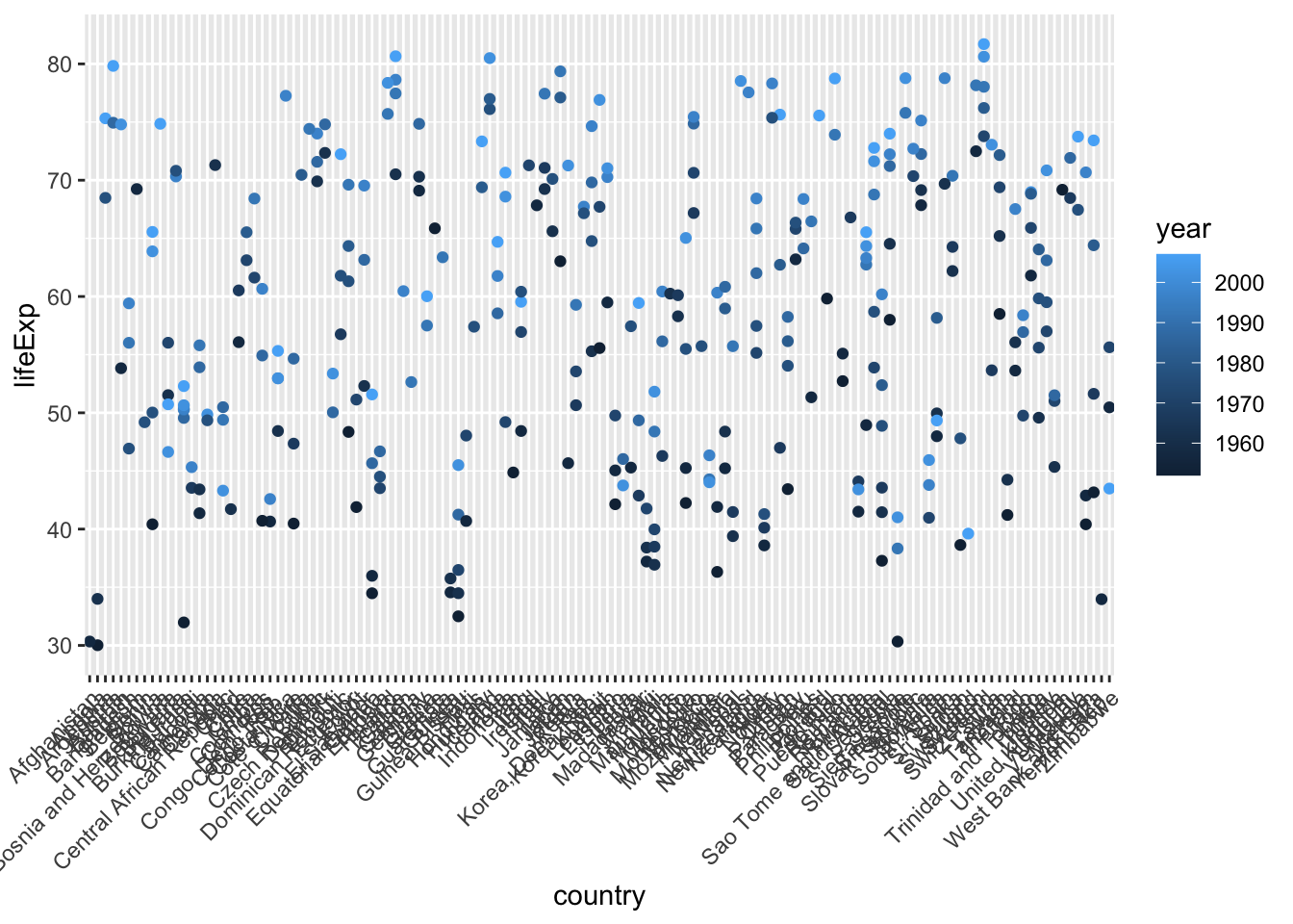
# plot just the most common ones
ggplot(mydata, aes(x=country_lump, y=lifeExp, color = year)) +
  geom_point() +
  theme(axis.text.x = element_text(angle = 45, vjust = 1, hjust=1))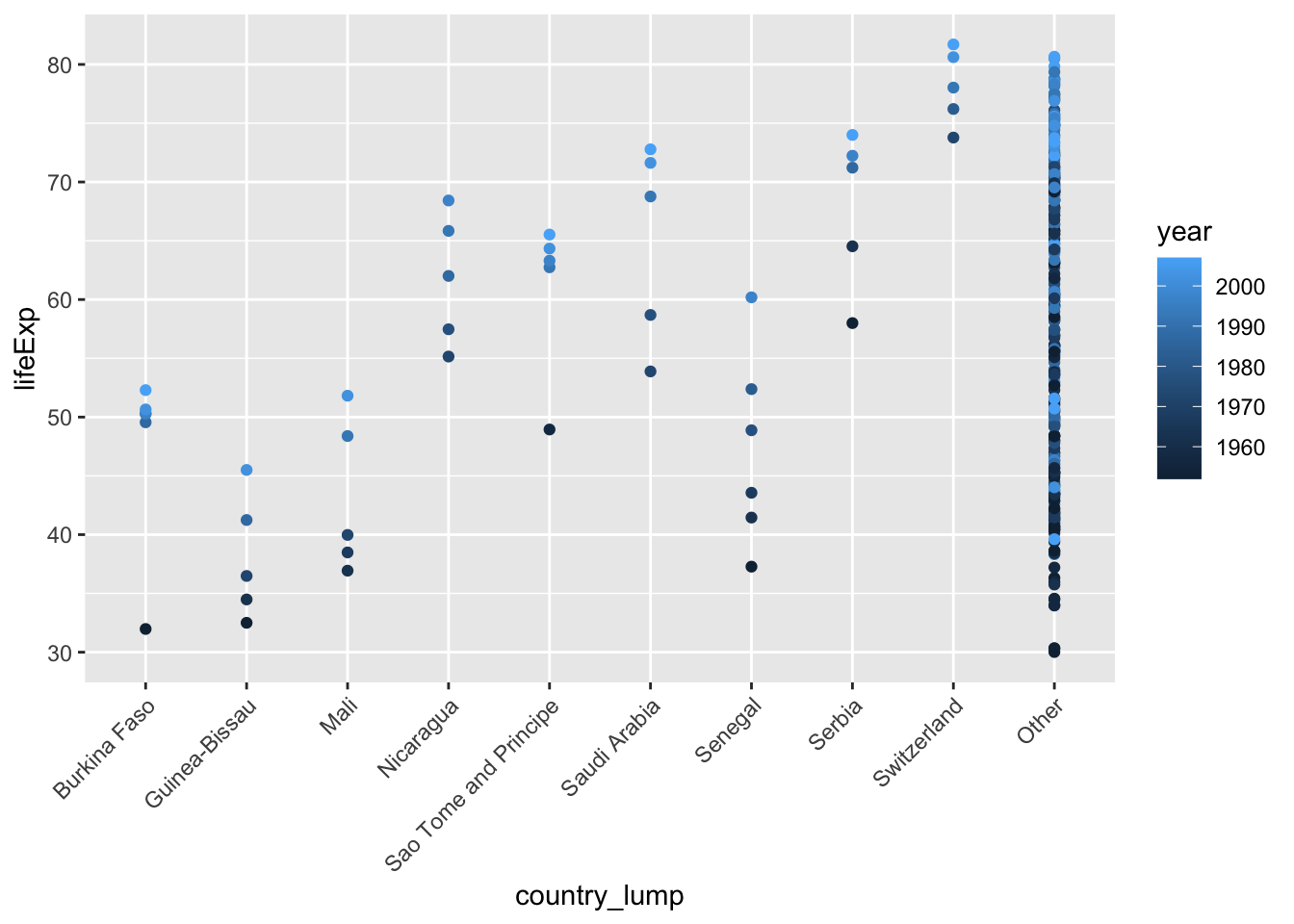
# remove the other category
ggplot(mydata %>% filter(country_lump!="Other"),
       aes(x=country_lump, y=lifeExp, color = year)) +
  geom_point() +
  theme(axis.text.x = element_text(angle = 45, vjust = 1, hjust=1))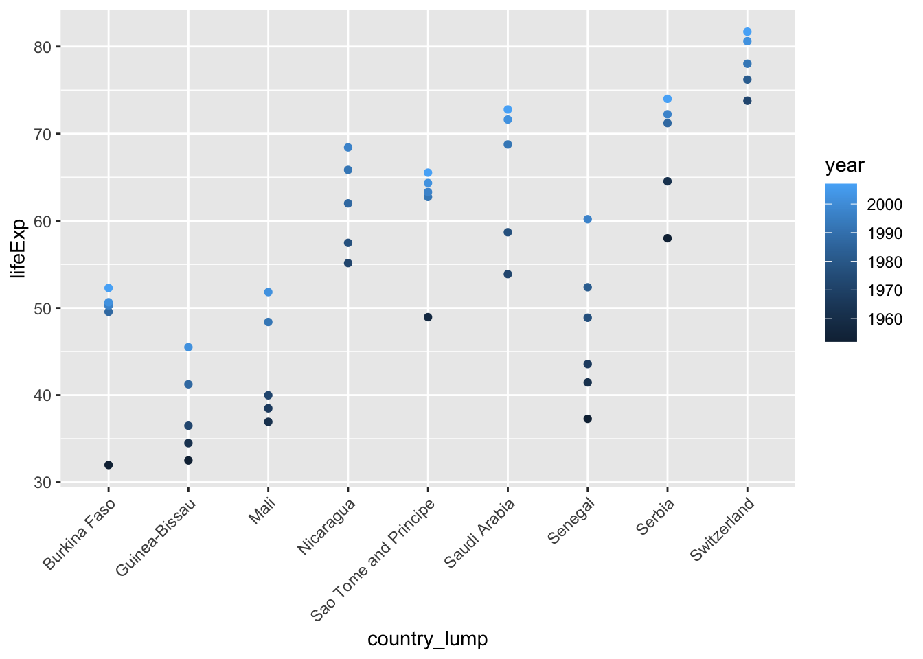
# plot in order of number of observations
levels(mydata$country_lump)
## [1] "Burkina Faso" "Guinea-Bissau" "Mali"
## [4] "Nicaragua" "Sao Tome and Principe" "Saudi Arabia"
## [7] "Senegal" "Serbia" "Switzerland"
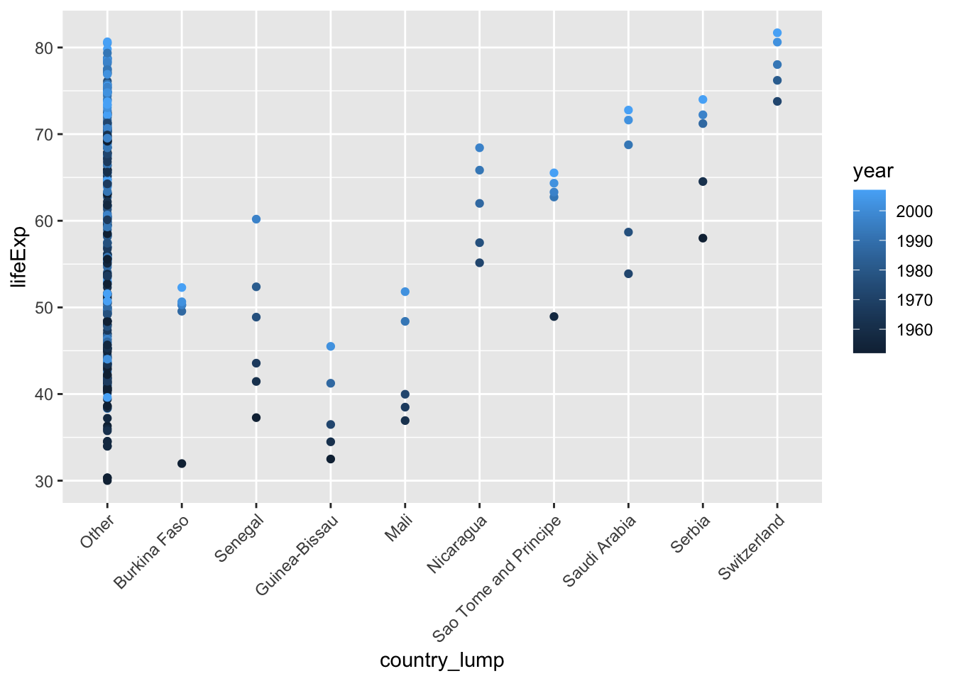
## [10] "Other"# this relevels the factor in order of frequency:
mydata <- mydata %>%
mutate(country_lump = fct_infreq(country_lump))
levels(mydata$country_lump)## [1] "Other" "Burkina Faso" "Senegal"
## [4] "Guinea-Bissau" "Mali" "Nicaragua"
## [7] "Sao Tome and Principe" "Saudi Arabia" "Serbia"
## [10] "Switzerland"# now plotting order has changed
ggplot(mydata, aes(x=country_lump, y=lifeExp, color = year)) +
geom_point() +
theme(axis.text.x = element_text(angle = 45, vjust = 1, hjust=1))