Part 3: ggplot2, factors, boxplots, dplyr: subsetting
R Project files
Please download the part3 folder from this dropbox folder link.
Use the grey “download” button to download the whole folder, please keep the file structure and folder organization exactly the same as we need this for class. Be sure to unzip if necessary. You may move the folder part3 wherever you like on your computer. Be sure to unzip if necessary.
In advance of class, please open the part3 Rstudio project (double click on the .rproj file), open part3.Rmd and knit (click the Knit button at the top of the file) this file. This will install packages that you need for the Rmd to run.
Readings
Required and suggested class readings can be found on the Readings tab by class. These readings may be done anytime before or after class, but they will supplement your understanding of the class materials and help make homework and project work easier.
Class Video
The class video is here, but I forgot to video tape the part about here::here(). If I have a chance I will re-record myself talking about it, but in the meantime, click here for Ted’s video from last year, start at linked time and watch for about 6 minutes, which explains similar ideas.
View last year’s class and materials here.
Post-Class
Please fill out the following survey and we will discuss the results during the next lecture. All responses will be anonymous.
- Clearest Point: What was the most clear part of the lecture?
- Muddiest Point: What was the most unclear part of the lecture to you?
- Anything Else: Is there something you’d like me to know?
Muddiest points
themes in ggplot
Check out this reference about ggplot themes first.
Here’s a couple examples using this one plot, so you can see how the theme changes the look of the figure, when you use built in themes from the ggplot2 package (yes it only works in ggplot figures, for the person who asked about that)
library(tidyverse)## ── Attaching packages ─────────────────────────────────────── tidyverse 1.3.2 ──
## ✔ ggplot2 3.3.6 ✔ purrr 0.3.4
## ✔ tibble 3.1.8 ✔ dplyr 1.0.9
## ✔ tidyr 1.2.0 ✔ stringr 1.4.0
## ✔ readr 2.1.2 ✔ forcats 0.5.1
## ── Conflicts ────────────────────────────────────────── tidyverse_conflicts() ──
## ✖ dplyr::filter() masks stats::filter()
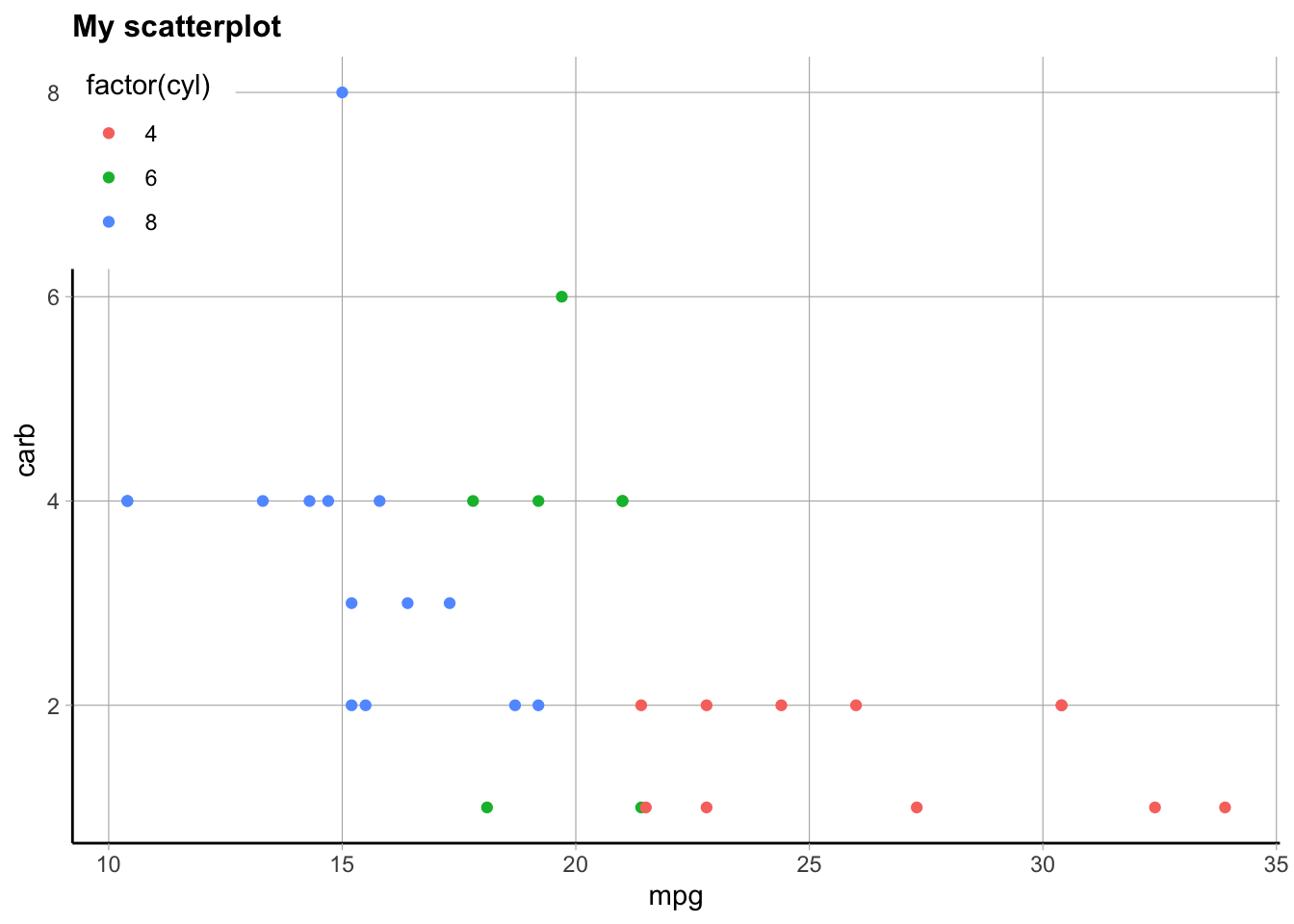
## ✖ dplyr::lag() masks stats::lag()p <- ggplot(mtcars, aes(x = mpg, y = carb, color = factor(cyl))) +
geom_point() +
labs(title = "My scatterplot")
p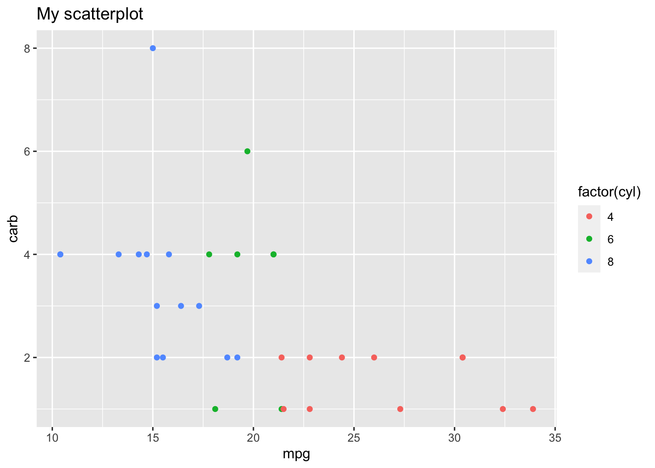
Here are some built in themes:
p + theme_bw()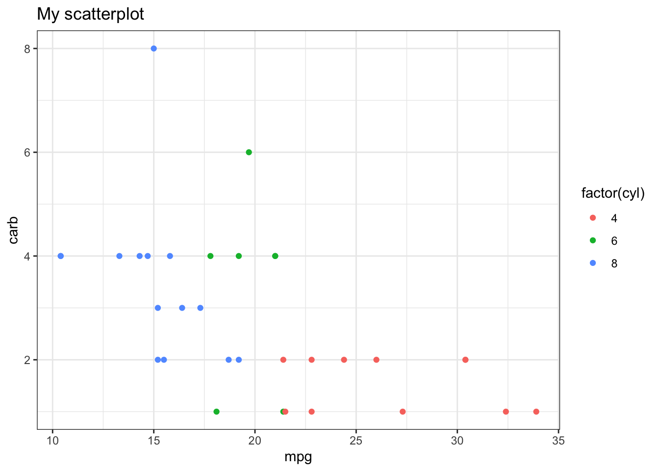
p + theme_minimal()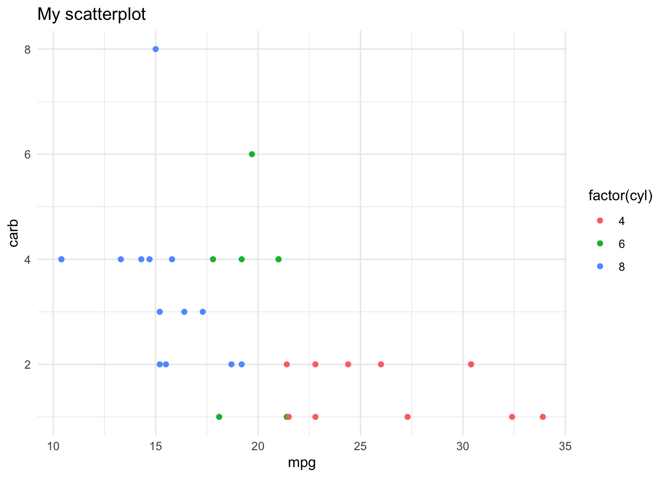
p + theme_classic()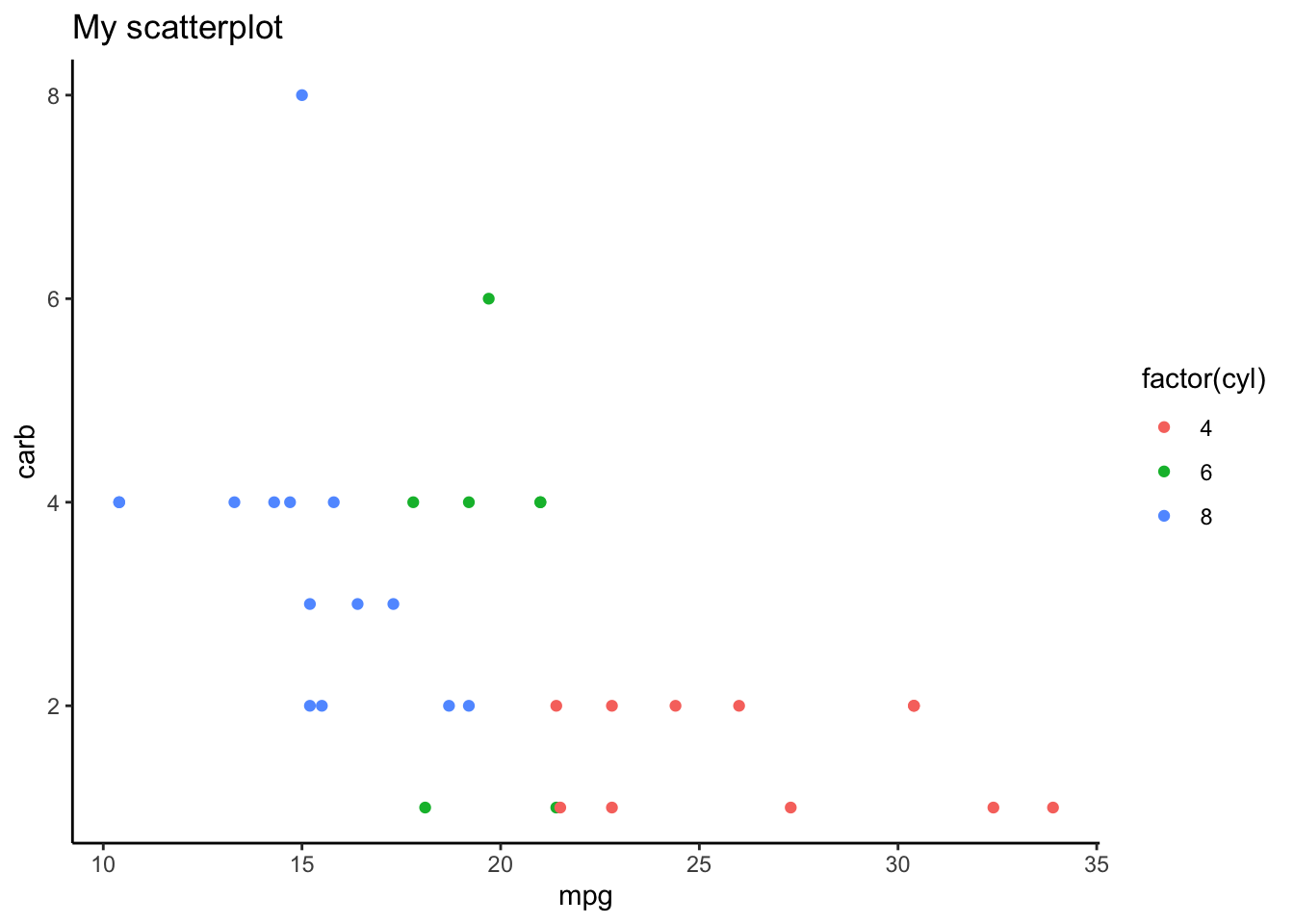
However you can make more customized themes or plot changes where you use the theme() function to add in a lot of other elements. You can use this add on function to choose specific parts of the plot that you want to change, like this example from the above reference. Anything specified here will override the built in theme selected first. There are many options, and looking at specific examples will help. I am always, always googling how to change parts of the theme/plot like this, because there are just so many options it’s too hard to remember them all.
p + theme_classic() +
  theme(
    plot.title = element_text(face = "bold", size = 12),
    legend.background = element_rect(fill = "white", size = 4, colour = "white"),
    legend.justification = c(0, 1),
    legend.position = c(0, 1),
    axis.ticks = element_line(colour = "grey70", size = 0.2),
    panel.grid.major = element_line(colour = "grey70", size = 0.2),
    panel.grid.minor = element_blank()
  )
Here’s a simpler example just changing the title (from the above reference):
p + theme(plot.title = element_text(size = 16))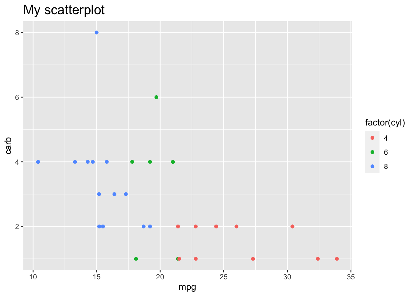
p + theme(plot.title = element_text(face = "bold", colour = "red"))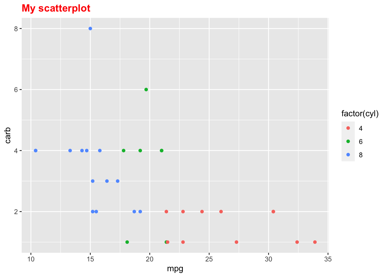
p + theme(plot.title = element_text(hjust = 1))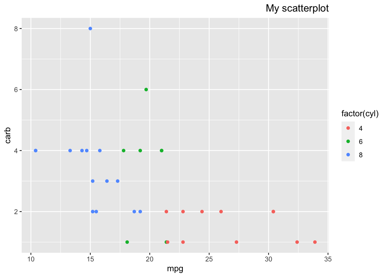
here()
Agreed, it’s very confusing, more in class 4!
Could you please clarify about the use of select(one_of) and the count command that was mentioned in dplyr cheatsheet?
These are very different, if you are talking about select() vs count(). One thing to note is that since I recorded that class, one_of() has been superseded/replaced by any_of() and all_of().
First, select() is a function to subset columns.
library(palmerpenguins)Here we specify the columns we want in the order we want:
penguins %>% select(bill_length_mm, island, species, year)## # A tibble: 344 × 4
## bill_length_mm island species year
## <dbl> <fct> <fct> <int>
## 1 39.1 Torgersen Adelie 2007
## 2 39.5 Torgersen Adelie 2007
## 3 40.3 Torgersen Adelie 2007
## 4 NA Torgersen Adelie 2007
## 5 36.7 Torgersen Adelie 2007
## 6 39.3 Torgersen Adelie 2007
## 7 38.9 Torgersen Adelie 2007
## 8 39.2 Torgersen Adelie 2007
## 9 34.1 Torgersen Adelie 2007
## 10 42 Torgersen Adelie 2007
## # … with 334 more rows
## # ℹ Use `print(n = ...)` to see more rowsHere, we pass a vector of character names, both of which work:
penguins %>% select(c("bill_length_mm","island","species","year"))## # A tibble: 344 × 4
## bill_length_mm island species year
## <dbl> <fct> <fct> <int>
## 1 39.1 Torgersen Adelie 2007
## 2 39.5 Torgersen Adelie 2007
## 3 40.3 Torgersen Adelie 2007
## 4 NA Torgersen Adelie 2007
## 5 36.7 Torgersen Adelie 2007
## 6 39.3 Torgersen Adelie 2007
## 7 38.9 Torgersen Adelie 2007
## 8 39.2 Torgersen Adelie 2007
## 9 34.1 Torgersen Adelie 2007
## 10 42 Torgersen Adelie 2007
## # … with 334 more rows
## # ℹ Use `print(n = ...)` to see more rowspenguins %>% select(any_of(c("bill_length_mm","island","species","year")))## # A tibble: 344 × 4
## bill_length_mm island species year
## <dbl> <fct> <fct> <int>
## 1 39.1 Torgersen Adelie 2007
## 2 39.5 Torgersen Adelie 2007
## 3 40.3 Torgersen Adelie 2007
## 4 NA Torgersen Adelie 2007
## 5 36.7 Torgersen Adelie 2007
## 6 39.3 Torgersen Adelie 2007
## 7 38.9 Torgersen Adelie 2007
## 8 39.2 Torgersen Adelie 2007
## 9 34.1 Torgersen Adelie 2007
## 10 42 Torgersen Adelie 2007
## # … with 334 more rows
## # ℹ Use `print(n = ...)` to see more rowsThis might be useful if we have that character vector already saved from some other data work we are doing:
colnames_needed <- c("bill_length_mm","island","species","year")
penguins %>% select(colnames_needed)
## Note: Using an external vector in selections is ambiguous.
## ℹ Use `all_of(colnames_needed)` instead of `colnames_needed` to silence this message.
## ℹ See <https://tidyselect.r-lib.org/reference/faq-external-vector.html>.
## This message is displayed once per session.## # A tibble: 344 × 4
## bill_length_mm island species year
## <dbl> <fct> <fct> <int>
## 1 39.1 Torgersen Adelie 2007
## 2 39.5 Torgersen Adelie 2007
## 3 40.3 Torgersen Adelie 2007
## 4 NA Torgersen Adelie 2007
## 5 36.7 Torgersen Adelie 2007
## 6 39.3 Torgersen Adelie 2007
## 7 38.9 Torgersen Adelie 2007
## 8 39.2 Torgersen Adelie 2007
## 9 34.1 Torgersen Adelie 2007
## 10 42 Torgersen Adelie 2007
## # … with 334 more rows
## # ℹ Use `print(n = ...)` to see more rowsBut the key about any_of and all_of is what it allows. any_of() allows column names that don’t exist! Using no tidyselect helper or all_of() does not allow this. Which you use depends on what you want to allow to happen.
colnames_needed <- c("bill_length_mm","island","species","year","MISSING")
# penguins %>% select((colnames_needed)) # does not work
penguins %>% select(any_of(colnames_needed)) # works!
## # A tibble: 344 × 4
## bill_length_mm island species year
## <dbl> <fct> <fct> <int>
## 1 39.1 Torgersen Adelie 2007
## 2 39.5 Torgersen Adelie 2007
## 3 40.3 Torgersen Adelie 2007
## 4 NA Torgersen Adelie 2007
## 5 36.7 Torgersen Adelie 2007
## 6 39.3 Torgersen Adelie 2007
## 7 38.9 Torgersen Adelie 2007
## 8 39.2 Torgersen Adelie 2007
## 9 34.1 Torgersen Adelie 2007
## 10 42 Torgersen Adelie 2007
## # … with 334 more rows
## # ℹ Use `print(n = ...)` to see more rows# penguins %>% select(all_of(colnames_needed)) # does not workany_of() is an example of a tidyselect helper, which we will see a lot more of when we start using across() with mutate() and summarize() in class 4. See this long list of useful tidyselect functions for more.
On the other hand, count() is mainly to count the number of unique values in a column/vector:
penguins %>% count(species)## # A tibble: 3 × 2
## species n
## <fct> <int>
## 1 Adelie 152
## 2 Chinstrap 68
## 3 Gentoo 124This created a new tibble, that summarizes the species column by counting the number of each type of species. This works for any type of vector but is most useful with character and factor columns. You can also use multiple columns here to see all possible combinations:
penguins %>% count(species, year)## # A tibble: 9 × 3
## species year n
## <fct> <int> <int>
## 1 Adelie 2007 50
## 2 Adelie 2008 50
## 3 Adelie 2009 52
## 4 Chinstrap 2007 26
## 5 Chinstrap 2008 18
## 6 Chinstrap 2009 24
## 7 Gentoo 2007 34
## 8 Gentoo 2008 46
## 9 Gentoo 2009 44Clearest Points
filter, select, arrange, pipes
Super! I want to take the time to mention (and hopefully not confuse everyone) that the pipe has recently (2021) been integrated into “base R”, that is, it’s loaded without loading the tidyverse package. HOWEVER it is this symbol |> and does not behave exactly like the tidyverse pipe %>% (actually from the magrittr package within the tidyverse package). For all the usual uses it works the same, so it could be used interchangeably in this class. Just know that if you see that type of pipe being used, assume it’s doing basically the same thing. Even R for Data Science is likely moving to use the native/base pipe, see this explanation. Probably next year’s class I will switch everything over to use this, though I still just use %>% in my own work as it’s slightly more flexible for more “advanced” usage.
penguins |> count(species, year)## # A tibble: 9 × 3
## species year n
## <fct> <int> <int>
## 1 Adelie 2007 50
## 2 Adelie 2008 50
## 3 Adelie 2009 52
## 4 Chinstrap 2007 26
## 5 Chinstrap 2008 18
## 6 Chinstrap 2009 24
## 7 Gentoo 2007 34
## 8 Gentoo 2008 46
## 9 Gentoo 2009 44Other messages
Density ridges are cool!
I agree!